How hashtags and captions change the perception and position of your brand on Instagram??
Using NLP to correlate the use of hashtags and captions for different fashion brands.
Hashtags are tags linked through different platforms. A proper hashtag is a visual component of an ad that can be used across different social networks to promote continuity of a campaign. Brands usually care about hashtags because these can reinforce a brand's position and promote customers' familiarity with it, which has an impact in the early stages of the buying cycle. But, can the use of hashtags (or captions) create an incorrect image of your brand? Let's say that you have a clothing brand in the category of designer, could the use of hashtags allude to another category of clothing?
My goal is to use NLP to find how the use of captions and hashtags on Instagram correlate across different brands and brand categories. I will use clustering, a machine learning unsupervised classification where no a priori knowledge (such as samples of classes) is assumed to be available.
The clustering task is grouping hashtags/captions in such a way that hashtags/captions in the same group (called a cluster) are more similar (in some sense) to each other than to those in other groups (clusters). Then I will analize how the clusters are associate with the different brands and categories, and how they affect engagement metrics.
My analysis consist of the next sections:
- Data description
- Text cleaning
- Kmeans model for hashtags
- Agglomerative clustering for hashtags
- Sentiment analysis of results
- Agglomerative clustering for captions
The data
I obtained the data from the project https://arxiv.org/abs/1704.04137. In their data project they obtained 24,752 Instagram posts by 13,350 people on Instagram through the Instagram’s API. The data collection was done over a month period in January 2015. And in all the posts renowned fashion brands are named in the hashtags.
The data includes:
- Basic information of the instagram account posting: Encrypted user id, amount of followers, amount of accounts following.
- Information about the post: Creation time of the post, engagement metrics (likes, comments), brand mentioned, captions, hashtags used.
- Learned features from their model (identifies the kind of picture).
- Learned features from Microsoft emotion API (identifies the emotion of the people that appears in the picture)
First step: installing all the packages and getting the data
I'm using python for this project.The nltk (the natural language toolkit) is a package of tools for working with text data. And scikit-learn for the machine learning models.
I donwloaded the data in a pandas dataframe, I will be working with the hashtags and captions but I'm keeping the columns of followers, likes and comments because I want to compare the different engagement metrics for the brand, brandcategories and clusters.
My first step was a simple formating (removing non-alphabetical characters and lowercasing) in the name of the columns and in the columns that includes the brandnames.
from ig_plotting import *
import nltk
from nltk.corpus import stopwords
import en_core_web_sm
from sklearn.feature_extraction import text
from sklearn.feature_extraction.text import TfidfVectorizer
from nltk.tokenize import RegexpTokenizer
from nltk.stem.snowball import SnowballStemmer
from sklearn.neighbors import LocalOutlierFactor
from sklearn.cluster import AgglomerativeClustering
import warnings
warnings.simplefilter(action='ignore', category=FutureWarning)
%matplotlib inline


#print('Loading words, spacy, punktd, stopwords')
nltk.download('words')
nlp = en_core_web_sm.load()
words = set(nltk.corpus.words.words())
nltk.download('stopwords')
#nltk.download('punkt')
print('done, now loading text and basic formating of columns name')


# Read dataset and format texts
df = pd.read_csv(r'fashion data on instagram.csv', index_col=0)#.sample(frac=0.2)

#Formating column names, brand categories names and brand names
df.columns = df.columns.str.strip().str.lower().str.replace(' ', '_').str.replace('-', '_').str.replace('?', '')
df.brandname = df.brandname.str.strip().str.lower().str.replace(' ', '_').str.replace('-', '_').str.replace('?', '')
df.brandcategory = df.brandcategory.str.strip().str.lower().str.replace(' ', '_').str.replace('-', '_').str.replace('?', '')
text_df = df[['brandcategory', 'hashtags', 'caption', 'brandname', 'comments', 'likes','followers']].copy(deep=True)
text_df = text_df[~text_df['hashtags'].isnull()]
text_df = text_df[~text_df['caption'].isnull()]
text_df = text_df[~text_df['followers'].isnull()]
brands = df.brandname.unique().tolist()
Text cleaning
First step is the text processing. The cleaning fuction takes all the entries in a column, removes the non-alphabetical characters, stopwords and encrypted words and returns the remaining text in lower cases.
The brand name was generated when the data was collected: A brand name used in fashion post search process, used as a hashtag in user’s post.
I removed from the hashatgs all the brands included in the brand category. If the brand appeared as a hashtag (Channel, Uniqlo, etc,.) my fuction replaces the hashtag with the word "brandname". If the hashtag was composed by a brandame an other word (Pradathailand, Dublindvf, etc,.), I replaced the hashtags with the word "brandreference". I think this is important because I didn't want the brand names as part of the corpus for my clusters (it would create noisy data and clusters correlated to brands heavily present in the dataset). But at the same time, I want to keep track of when a brand name is used as any kind hashtag.
** I removed only the brands presented in the brand column.
I also have the tokenize function that I will call later with TfidVectorizer. Tokenize takes the text entries, extracts the words and reduce them to their roots.
import re
def cleaning(frame,col):
    """
    Function to clean text from a column in a data frame

    This funtion removes non alphabethic characters,stop words and numerical characters and return text in lowers.

    Parameters:
    Data frame, text column

    Returns:
    values clean text from column

    """
    newframe=frame.copy()
    newframe=newframe[~newframe[col].isnull()]
    punc = ['.', ',', '"', "'", '?', '!', ':', ';', '(', ')', '[', ']', '{', '}','#',"%"]
    stop_words = text.ENGLISH_STOP_WORDS.union(punc)
    stop_words = list(stop_words)
    newframe[col]=newframe[col].str.replace('\d+', '').str.replace('\W', ' ').str.lower().str.replace(r'\b(\w{1,3})\b', '')
    newframe[col] = [' '.join([w for w in x.lower().split() if w not in stop_words]) for x in newframe[col].tolist()]
    newframe[col] =[' '.join(word for word in x.split() if not word.startswith('uf')if not word.startswith('ue')if not word.startswith('u0')) for x in newframe[col].tolist()]

    newframe[col] =[' '.join([word,'brandname'][word in brands] for word in x.split()) for x in newframe[col].tolist()]
    newframe[col] =[' '.join([word,'brandreference'][word.startswith(tuple(brands))] for word in x.split()) for x in newframe[col].tolist()]
    newframe['Cleantext'] =[' '.join([word,'brandreference'][word.endswith(tuple(brands))] for word in x.split()) for x in newframe[col].tolist()]

    content = newframe['Cleantext']#.values
    return content

stemmer = SnowballStemmer('english')
tokenizer = RegexpTokenizer(r'[a-zA-Z\']+')

def tokenize(text):
    return [stemmer.stem(word) for word in tokenizer.tokenize(text)]
clean_hashtags = cleaning(text_df,'hashtags')
text_df['clean_hashtags'] = clean_hashtags
Now I will conver my text to a matrix of TF-IDF features using TdifVectorizer. TdifVectorizer takes the corpus as input and make the following steps:
- Make an ordered list of all the words in the corpus, commonly referred to as a dictionary or the vocabulary.
- For each document, count the number of times a word in the vocabulary appears in the document and applies some extra weighting to the counts.
- It creates a tfidf matrix with all the words and their scores in all the text. The fit_transform() method above converts the list of strings to a sparse matrix. In this case, the matrix represents tf-idf values for all texts.
vectorizing = TfidfVectorizer(sublinear_tf=True,  min_df=100, norm='l2',
                              ngram_range=(1, 1), tokenizer = tokenize)

%time clean_hashtags_vector = vectorizing.fit_transform(clean_hashtags.values) #fit the vectorizer
#terms = vectorizing.get_feature_names()
#print(len(terms))
Outliers treatment
Clustering algorithms are sensitive to outliers in the data set, and outlier detection is more difficult when doing unsupervised clustering since I am trying to learn what the clusters are, and what data points correspond to "no" clusters.
I'm going to use LocalOutlierFactor to identify the outliers and then trimmer the data. LocalOutlierFactor is an unsupervised outlier datector. The outlier score measures the local deviation of density of a given sample with respect to its neighbors, the score depends on how isolated the object is with respect to the surrounding neighborhood.
By comparing the local density of a sample to the local densities of its neighbors, I can identify samples that have a substantially lower density than their neighbors, and these are considered outliers. The number of neighbors that I will use to compare is 50. The negative outlier factor captures the degree of abnormality, the closer to -1 the more normal is the data point, and the outliers have smaller factors. I kept the points with an outlier factor of -5 or higher. I did this because in a previous analysis, and failed attempts to cluster, I found data points with a negative outlier factor were messing with the clustering.
def filterbyoutlier(df,vector):
    clfhash = LocalOutlierFactor(n_neighbors=50)
    clfhash.fit_predict(vector.toarray())
    df['outlier_factor_hash'] = clfhash.negative_outlier_factor_
    return df[df['outlier_factor_hash']>-5]
data = filterbyoutlier(text_df, clean_hashtags_vector)
clean_hashtags_vector = vectorizing.fit_transform(cleaning(data,'hashtags').values)
Kmeans.
Kmeans is a widely used method in cluster analysis. You select the number of clusters, k, and the algorithm which minimizes the sum of squared errors (SSE), the within cluster squared error.
To select the number of cluster we can use the elbow method; it runs k-means clustering on the dataset for a range of values for k (say from 1-100) and then for each value of k computes the SSE score for all clusters. The line chart resembles an arm, then the “elbow” (the point of inflection on the curve), and at that point the model fits best.
I found the elbow at 5. And then I found the 5 clusters for the hastags. However, the disadvantage of kmeans is that is designed for clustering spherical groups of equal size and variance. This is not reliable for our real data, so I will use agglomerative clustering to look for clusters in the next step. But I included the kmeans results in this analysis.
finding_k(clean_hashtags_vector,1, 40,5, "Elbow plot")

kmeans_hashtags = KMeans(n_clusters = 5, n_jobs = -1, max_iter=10, random_state=True, n_init=50)
kmeans_hashtags.fit(clean_hashtags_vector)
data['kcluster_hashtags'] = kmeans_hashtags.labels_
My function plotclusterscorr plots the correlation of each cluster to brandcategory/brandname. (All the plotting functions are included in ig_plotting.py.
plotclusterscorr(data,'brandcategory','kcluster_hashtags')

All the brandcategories are correlated with clusters 0 and 2. And megacouture is strongly correlated with cluster 1.
Now I will visualize the brands are within each cluster. The size in the brandname in the cloud function depends of the frequency that brand was classified in the cluster, each brand category has a color:
- Designer brands are in blue.
- Small couture brands are green.
- High street brands are purple.
- Megacouture brands are in orange.
cloudgenerator(5, data, 'kcluster_hashtags')


In the cluster 0 we see a variety of designer, highstreet and small couture brands. Brands like Cesare Attonlini, Zara, DVF, Calvin Klein, Vince, Iro and Nancy Gonzalez are the most present in the cluster. It's very interesting that this brands share hashtagas but their target customer are different.
From the wordclouds we can see that Loropiana, Fabianafilippi and Brunello Cucinelli (small couture brands) belong to cluster 1.
In the cluster 2 we see a variety of designer, highstreet and small couture brands. The most present brands are Viviene Westwood, Theory and Ermenegildo Zegna.
In the cluster 3 we see designer, small and mega coture brands. And in cluster 4 are designer, high street and megac couture brands, and the most present brands are Prada and Kate Spade.
list1 = [50,100,500,1000,2000,10000]
dict_clusters = {0:"gold", 1:'darkcyan', 2:'plum', 3:'royalblue', 4:'salmon'}
interact(plotjoint, df=fixed(data), clusters=fixed('kcluster_hashtags'), color_code=fixed(dict_clusters), x_col=fixed('likes'),
         y_col=fixed('comments'), xlim=list1, ylim=list1, atitle=fixed("Dist hashtags clusters"))
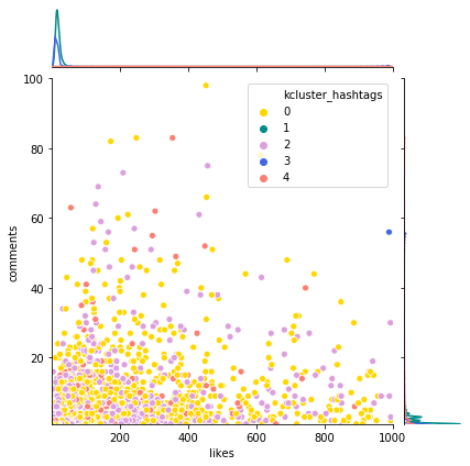
From the kde plots we can see that clusters 1 and 3 have a higher mean and smaller variance. But this can be caused by the cluster size. To understand better I will summarize the data available for the clusters.
df1 = data.groupby(['kcluster_hashtags'])[['comments','likes', 'followers']].mean().rename(columns={'likes':'Avg Likes', 'comments':'Avg Comments', 'followers':'Avg Followers'})
df1['Avg likes per followers'] = df1['Avg Likes']/df1['Avg Followers']
df1['Avg comments per followers'] = df1['Avg Comments']/df1['Avg Followers']
df2 = data.groupby(['kcluster_hashtags']).size().to_frame('cluster size')
kmetrics = pd.concat([df1, df2], axis=1, sort=False)
kmetrics
We can see that cluster 0 has the largest size and group 1 the smallest. Group 1 has the highest engagement in the posts, and cluster 3 has the smallest engagement metrics, even when cluster 4 has the lowest average of users.
clusterwords(clean_hashtags_vector,vectorizing,kmeans_hashtags)
The top ten words in every cluster are presented in the dataframe above. First interesting thing is that all the clusters except cluster 1 include a lot of selfreference to the brand.
Also other brands that were not included in the brand column are present in the clusters, for example: Valentino, Dior, MiuMiu, Fendi, Celine, Dolce and Gabbana and Givenchi are presented in cluster 3. All these are megacoture brands, and indicates that people wear two or more megacouture brands at the same time.
Agglomerative clustering
It's an algorithm that recursively merges the pair of clusters that minimally increases a given linkage distance.
Hierarchical clustering is a better option than kmeans. You don't need to make assumptions about the distribution of your data, the only requirement (which k-means also shares) is that a distance can be calculated each pair of data points.
The parameters for this algorithm are:
- The number of clusters to find.
- The affinity or metric to measure distance.
- The linkage parameter to determine the merging strategy to minimize.
The ward method minimizes the variance of merged clusters, Ward is the most effective method for noisy data https://scikit-learn.org/stable/auto_examples/cluster/plot_linkage_comparison.html.
Number of clusters
Now, I need to find the number of clusters that we want our data to be split. I'm using the scipy library to create the dendrograms for our dataset. The hierarchy class of the scipy.cluster library has a dendrogram method which takes the value returned by the linkage method of the same class. The linkage method takes the dataset and the method to minimize distances as parameters. I followed this method to find the number of clusters https://stackabuse.com/hierarchical-clustering-with-python-and-scikit-learn/.
print('Generating dendrogram...')
#import scipy.cluster.hierarchy as shc

#plt.figure(figsize=(10, 7))
#plt.title("Hashtag Dendograms")
#dend = shc.dendrogram(shc.linkage(clean_hashtags_vector.toarray(), method='ward'))
Generating dendrogram...
If I draw a horizontal line that passes through longest distance without a horizontal line, I got 8 clusters.
Clusters
Now, I call the agglomerative clustering algorithm in sklearn and find the clusters.
cluster = AgglomerativeClustering(n_clusters=7, affinity='euclidean', linkage='ward')
cluster.fit_predict(clean_hashtags_vector.toarray())
data['hashtags_clusters'] = cluster.labels_
plotclusterscorr(data,'brandcategory','hashtags_clusters')

For this model we see that all the brand categories are correlated with ckuster 0.
Small couture is the only brand correlated to cluster 1 and 4.
Mega couture is the only correlated to cluster 5.
cloudgenerator(7, data, 'hashtags_clusters')


Again the color code is:
- Designer brands are in blue.
- Small couture brands are green.
- High street brands are purple.
- Megacouture brands are in orange.
In cluster 0 we see a variety of designer, small couture and high street brands. With Calvin Klein, DVF, Vince and Cesare Atolinni are the most present brands.
In cluster 1 we see two small couture brands: Loropiano and Brunello Cucinnelli.
In cluster 2 we see a variety of the four categories, the most present are: Kate Spade and Topshop.
In cluster 3 we see a variety of designer, small couture and high street brands. But the most present brands are Vivienne Westwood, Vince and Theory.
In cluster 4 just Fabian Filipi is presented.
In cluster 5 two megacouture brands are presented: Prada and Hermes.
list1 = [50,100,500,1000,2000,10000]
dict_clusters={0:"gold", 1:'darkcyan', 2:'plum', 3:'royalblue', 4:'salmon', 5:'pink', 6:'steelblue', 7:'orchid'}
interact(plotjoint, df=fixed(data), clusters=fixed('hashtags_clusters'), color_code=fixed(dict_clusters), x_col=fixed('likes'),
         y_col=fixed('comments'), xlim=list1, ylim=list1, atitle=fixed("Dist hashtags clusters"))
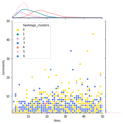
df1 = data.groupby(['hashtags_clusters'])[['comments','likes', 'followers']].mean().rename(columns={'likes':'Avg Likes', 'comments':'Avg Comments', 'followers':'Avg Followers'})
df1['Avg likes per followers'] = df1['Avg Likes']/df1['Avg Followers']
df1['Avg comments per followers'] = df1['Avg Comments']/df1['Avg Followers']
df2 = data.groupby(['hashtags_clusters']).size().to_frame('cluster size')
aggmetrics = pd.concat([df1, df2], axis=1, sort=False)
aggmetrics
Cluster 0 has the highest engagement metrics by follower.
clusterwords(clean_hashtags_vector,vectorizing,cluster)
In all the clusters except 1 we see a lot of brands self-references. We see a lot of references to brands not included in the brand column and also a lot of reference to places like Switzerland, Singapore and Paris.
Hashtags results
For the final analysis I want to study how the emotions in the hashtags affect the engagement metrics. For this I will use sentiment analysis with TextBlob.
TextBlob is an open source python library used for textual analysis. It is very much useful in Natural Language Processing and Understanding.
There are two things that we can measeure:
- Polarity
- Subjectivity
Polarity
Polarity helps us in finding the expression and emotion of the author in the text. The value ranges from -1.0 to +1.0 and they contain float values.
- Less than 0 denotes Negative
- Equal to 0 denotes Neutral
- Greater than 0 denotes Positive
Values near to +1 are more likely to be positive than a value near to 0. Same is in the case of negativity.
Subjectivity
It tell us if a sentence is subjective or objective. The value ranges from 0.0 to +1.0
Subjective sentences are based on personal opinions, responses, beliefs whereas objective sentences are based on factual information.
First analyzing for the kmeans clusters
I created a data frame that includes metrics and the sentiment analysis for each cluster
** Analysis function is inside of ig_plotting.py
The polarity and subjectivity values are neutral, this is due that usually hastags in a post are just words. I got better values for the captions since they are sentences.
Cluster 0 and 4 have the highest values for polarity and subjectivity.
kmsens = pd.concat((data['kcluster_hashtags'],analysis(data, 'clean_hashtags', 'hashtags_polarity','hashtags_subjectivity')), axis=1, sort=False).groupby(['kcluster_hashtags'])[['hashtags_polarity','hashtags_subjectivity']].mean()
kmsens = pd.concat((kmsens, kmetrics[['Avg comments per followers','Avg likes per followers']]), axis=1, sort=False)
kmsens
Now analyzing the correlation we see a high correlation between the metrics and polairyt and subjectivity.
kmsens.corr()
Analyzing for the agglomerative clusters
aggsens = pd.concat((data['hashtags_clusters'],analysis(data, 'clean_hashtags', 'hashtags_polarity','hashtags_subjectivity')), axis=1, sort=False).groupby(['hashtags_clusters'])[['hashtags_polarity','hashtags_subjectivity']].mean()
aggsens = pd.concat((aggsens, aggmetrics[['Avg comments per followers','Avg likes per followers']]), axis=1, sort=False)
aggsens
aggsens.corr()
Agglomerative clustering for captions.
First I repeated the same process that I did we hashtags: cleaning of the caption column, remove outliers and then use a dendogram to find the number of clusters.
clean_captions = cleaning(text_df,'caption')
text_df['clean_captions'] = clean_captions
%time clean_captions_vector = vectorizing.fit_transform(clean_captions.values)
data=filterbyoutlier(text_df, clean_captions_vector)
clean_captions_vector = vectorizing.fit_transform(cleaning(data,'caption'))
#plt.figure(figsize=(10, 7))
#plt.title("Caption Dendograms")
#dend = shc.dendrogram(shc.linkage(clean_captions_vector.toarray(), method='ward'))
If I draw a horizontal line that passes through longest distance without a horizontal line, I get 5 clusters as shown in the following above. Then I ran the model and got the labels.
clustercap = AgglomerativeClustering(n_clusters=6, affinity='euclidean', linkage='ward')
clustercap.fit_predict(clean_captions_vector.toarray())
data['captions_clusters'] = clustercap.labels_
plotclusterscorr(data,'brandcategory','captions_clusters')

cloudgenerator(6, data, 'captions_clusters')


Add text after running
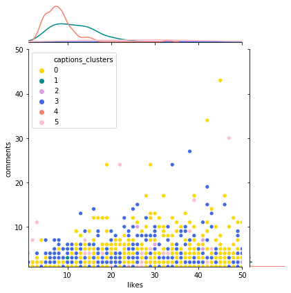
list1 = [50,100,500,1000,2000,10000]
dict_clusters = {0:"gold", 1:'darkcyan', 2:'plum', 3:'royalblue', 4:'salmon', 5:'pink', 6:'steelblue'}
interact(plotjoint, df=fixed(data), clusters=fixed('captions_clusters'), color_code=fixed(dict_clusters), x_col=fixed('likes'),
         y_col=fixed('comments'), xlim=list1, ylim=list1, atitle=fixed("Dist captions clusters"))
clusterwords(clean_captions_vector,vectorizing,clustercap)
# Sentiment analysis
aggsens = pd.concat((data['captions_clusters'],analysis(data, 'clean_captions', 'hashtags_polarity','hashtags_subjectivity')), axis=1, sort=False).groupby(['captions_clusters'])[['hashtags_polarity','hashtags_subjectivity']].mean()
aggsens = pd.concat((aggsens, aggmetrics[['Avg comments per followers','Avg likes per followers']]), axis=1, sort=False)
aggsens
aggsens.corr()