Back to main page

Predicting Hotel Booking Conversion Rates in Real Zero-Inflated Data: A Dual-Model Approach

Trivago is a meta-search website that enables advertisers to promote accommodations and allows users to compare different prices for the same accommodation. By aggregating offers from various booking sites, Trivago provides users with a comprehensive view of available options, helping them to make informed decisions and find the best deals.

The task given was to create a model to predict conversion rates for hotel bookings across various advertising sites. This involved using the provided anonymized real data to make predictions for each advertiser-hotel combination for the specific date of August 11. The challenge was further compounded by the sparsity of data and the presence of zero-inflated data, as many advertiser-hotel combinations had no bookings at all.

Data Available

Two datasets are provided for this case study:

1. hotels.csv
   • hotel_id: Unique identifier of a given accommodation.
   • stars: Number of stars of the corresponding hotel.
   • rating: Average rating given by users on a scale from 0 to 10.
   • n_reviews: Number of reviews used to calculate the rating.
   • city_id: Unique identifier of the city where the hotel is locate.
2. metrics.csv
   • ymd: Date in YYYYMMDD format.
   • hotel_id: Unique identifier of a given accommodation.
   • advertiser_id: Unique identifier of the advertiser.
   • n_clickouts: Number of clicks from users on a particular hotel item from a specific advertiser on a given day.
   • n_bookings: Number of bookings made by users for a particular hotel item from a specific advertiser on a given da

Goals

• Focus on overcoming the challenge of data sparsity and develop model to predict the conversion rate.
• Use the developed model to predict the conversion rate for each advertiser-hotel combination on the next day, August 11.

import numpy as np
import pandas as pd
import scipy.stats as stats
import matplotlib.pyplot as plt
import seaborn as sns
import matplotlib.dates as mdates
from matplotlib.gridspec import GridSpec
#sns.set_theme(style='whitegrid')
sns.set_theme()

from xgboost import XGBClassifier, XGBRegressor
from sklearn.model_selection import train_test_split, GridSearchCV
from sklearn.utils.class_weight import compute_sample_weight
from sklearn.metrics import make_scorer, precision_score, recall_score, accuracy_score
pd.options.mode.chained_assignment = None  
pd.set_option('display.max_rows', 8)

Hotels

The descriptive analytics of the hotels data reveal that the dataset consists of 224 rows, all numeric despite containing categorical information. Additionally, hotel 216 is noted for having missing data in both n_reviews and rating fields based on the information provided.

After refining the column types, such as categorizing city_id, hotel_id, and stars appropriately, I delved into a detailed analysis of both categorical and numerical variables, uncovering compelling insights:

Each row in the dataset corresponds to a unique hotel, offering a diverse range of insights into the hospitality landscape.

Among the six different star categories, 4-star hotels emerge as the most prevalent, constituting 33.93% of the dataset and reflecting a popular choice among travelers.

Spanning across 86 distinct cities, city_id 34 emerges as a focal point, hosting 13.84% of all hotels and showcasing a significant presence in the dataset.

The average number of reviews per hotel (n_reviews) stands at 2960, with a standard deviation of 3880, indicating varied engagement levels among guests and a distribution skewed towards highly reviewed establishments.

Hotels maintain an average rating of 7.87, with a standard deviation of 1.05, reflecting a generally positive sentiment but with notable variation and a distribution skewed towards higher ratings.

hotels = pd.read_csv('data/hotels.csv')
print(hotels.info())
print('The hotel with null info:\n ',hotels[hotels.isnull().any(axis=1)])

<class 'pandas.core.frame.DataFrame'>
RangeIndex: 224 entries, 0 to 223
Data columns (total 5 columns):
 #   Column     Non-Null Count  Dtype  
---  ------     --------------  -----  
 0   hotel_id   224 non-null    int64  
 1   stars      224 non-null    int64  
 2   n_reviews  223 non-null    float64
 3   rating     223 non-null    float64
 4   city_id    224 non-null    int64  
dtypes: float64(2), int64(3)
memory usage: 8.9 KB
None
The hotel with null info:
       hotel_id  stars  n_reviews  rating  city_id
215       216      0        NaN     NaN        3

def df_insights(df):
    df_numerical_features = df.select_dtypes(include=['number']).columns.tolist()
    df_categorical_features = df.select_dtypes(include=['category']).columns.tolist()
    print('For df data frame of size ',len(df),' we have :')
    for col in df_categorical_features:
        print('\n-  For "',col,'" there are ', df[col].nunique(),' unique values')
        if df[col].nunique()!=len(df):
            print('   The most common value is "', df[col].mode()[0],'" with ',
                  '{:.2f}'.format(len(df[df[col]==df[col].mode()[0]])*100/len(df)),'%')
            
    for col in df_numerical_features:
        print('\n-  For "',col,'" there are ', df[col].nunique(),' unique values')
        print('   The avg value is ', '{:.2f}'.format(df[col].mean()),' with ',
                  '{:.2f}'.format(df[col].std()),'sdv, and', '{:.2f}'.format(df[col].skew(axis = 0, skipna = True)), 'skew.') 

hotels['city_id'] = hotels['city_id'].astype('category')
hotels['hotel_id'] = hotels['hotel_id'].astype('category')
hotels['stars'] = hotels['stars'].astype('category')        
#df_insights(hotels)

For df data frame of size  224  we have :

-  For " hotel_id " there are  224  unique values

-  For " stars " there are  6  unique values
   The most common value is " 4 " with  33.93 %

-  For " city_id " there are  86  unique values
   The most common value is " 34 " with  13.84 %

-  For " n_reviews " there are  218  unique values
   The avg value is  2960.43  with  3889.41 sdv, and 3.00 skew.

-  For " rating " there are  45  unique values
   The avg value is  7.87  with  1.05 sdv, and -1.17 skew.

The majority of hotels in the dataset boast a 4-star rating, suggesting a popular choice among guests. Interestingly, hotels rated 4, 5, and surprisingly, 1 star, tend to receive the highest ratings, indicating exceptional guest satisfaction across different luxury levels.

However, hotels with a 1-star rating notably receive fewer reviews compared to their higher-star counterparts, hinting at potential differences in guest interaction and overall visibility within the dataset.

These insights underscore how star categories not only influence perceptions of quality but also shape guest engagement metrics in the hospitality industry.

n_hotels_stars = hotels[['hotel_id','stars']].groupby('stars').count().reset_index().rename(columns={'hotel_id': 'number_hotels'})
n_hotels_stars = n_hotels_stars.sort_values(by='number_hotels', ascending=False)

cmap = plt.cm.RdYlGn
colors = [cmap(i / 6) for i in range(6)]
color_dict = {i: colors[i] for i in range(6)}

g = sns.catplot( data=n_hotels_stars, kind='bar', x='stars',  y='number_hotels', order = n_hotels_stars['stars'],
               height=2.5, aspect=8/2.5, palette=color_dict)

g.fig.suptitle('Number of hotels per stars', y=1.01)
#g.set_xticklabels(rotation=90)

fig, axes = plt.subplots(1,2, figsize=(9,2.5))

sns.boxplot(data=hotels, y='rating', x='stars', palette=color_dict, ax=axes[0], order = n_hotels_stars['stars'])
sns.boxplot(data=hotels, y='n_reviews', x='stars', palette=color_dict, ax=axes[1], order = n_hotels_stars['stars'])
plt.subplots_adjust(wspace=0.5)
axes[0].set_title('Rating per star category')
axes[1].set_title('N. reviews per star category')

C:\Users\thalia\anaconda3\envs\assignmet_june24\lib\site-packages\seaborn\axisgrid.py:118: UserWarning: The figure layout has changed to tight
  self._figure.tight_layout(*args, **kwargs)

Text(0.5, 1.0, 'N. reviews per star category')

Metrics

The metrics dataset comprises a substantial 10,292 rows, all with typea numeric despite encompassing categorical variables. Impressively, this dataset exhibits a complete absence of null values, ensuring robustness and reliability in the analytical process. These characteristics not only underscore the dataset's integrity but also pave the way for comprehensive exploratory analyses to uncover deeper patterns and relationships within the metrics of hotel interactions.

This dataset has undergone significant enhancements to prepare it for thorough analysis:

• Column types, including hotel_id and advertising_id, were accurately categorized.
• Dates were standardized using pandas.datetime for consistency.
• Day of the week was extracted to capture shopping trends, categorizing entries from Monday through Sunday.
• The crucial C2B column, representing the percentage of clickouts that led to bookings, was computed.
• A new combined column of advertiser_id and hotel_id was introduced to facilitate predictive feature engineering.

Key insights from the analysis reveal:

• The dataset includes 224 unique hotels, with hotel 36 being the most prevalent at 1.21%.
• There are 43 distinct advertisers, with advertiser 5 appearing in 19% of entries.
• Wednesdays dominate as the most common day, representing 20% of entries.
• The dataset contains 2,040 unique hotel-advertiser combinations, with hotel 1 and advertiser 5 being the most frequent at 0.1%.
• On average, entries have 13.39 clickouts with a standard deviation of 41.
• The average number of bookings per entry is 0.33, with a standard deviation of 1.25.
• The average conversion rate (C2B) stands at 2.41%, with a standard devinds and patterns.

metrics = pd.read_csv('data/metrics.csv')
metrics.info()

<class 'pandas.core.frame.DataFrame'>
RangeIndex: 10292 entries, 0 to 10291
Data columns (total 5 columns):
 #   Column         Non-Null Count  Dtype
---  ------         --------------  -----
 0   ymd            10292 non-null  int64
 1   hotel_id       10292 non-null  int64
 2   advertiser_id  10292 non-null  int64
 3   n_clickouts    10292 non-null  int64
 4   n_bookings     10292 non-null  int64
dtypes: int64(5)
memory usage: 402.2 KB

metrics['hotel_id'] = metrics['hotel_id'].astype('category')
metrics['advertiser_id'] = metrics['advertiser_id'].astype('category')
#Format date
metrics['ymd'] = pd.to_datetime(metrics['ymd'], format='%Y%m%d')
# Get the day of the week name
metrics['day_of_week'] = metrics['ymd'].dt.day_name()
metrics['day_of_week'] = metrics['day_of_week'].astype('category')
metrics['C2B'] = 100*metrics['n_bookings']/metrics['n_clickouts']
metrics['hotel_adv_combination'] = metrics['hotel_id'].astype(str)+'-'+metrics['advertiser_id'].astype(str)
metrics['hotel_adv_combination'] = metrics['hotel_adv_combination'].astype('category')

#df_insights(metrics)       

For df data frame of size  10292  we have :

-  For " hotel_id " there are  224  unique values
   The most common value is " 36 " with  1.21 %

-  For " advertiser_id " there are  43  unique values
   The most common value is " 5 " with  18.99 %

-  For " day_of_week " there are  7  unique values
   The most common value is " Wednesday " with  20.61 %

-  For " hotel_adv_combination " there are  2040  unique values
   The most common value is " 1-5 " with  0.10 %

-  For " n_clickouts " there are  234  unique values
   The avg value is  13.39  with  41.08 sdv, and 10.56 skew.

-  For " n_bookings " there are  24  unique values
   The avg value is  0.33  with  1.25 sdv, and 9.29 skew.

-  For " C2B " there are  337  unique values
   The avg value is  2.41  with  9.79 sdv, and 7.11 skew.

There is no correlation between the number of hotels per advertiser and their respective clickouts and bookings. Notably, advertisers 5 and 43 lead in both clickouts and bookings.

Interestingly, advertiser 43 promotes only one hotel, namely hotel 141. However, hotel 141 is also advertised by 7 other advertisers

metrics['log_C2B'] = np.log10(metrics[['C2B']]+1)
metrics['log_n_bookings'] = np.log10(metrics['n_bookings']+1 )
metrics['log_n_clickouts'] = np.log10(metrics['n_clickouts'] +1)

n_hotels_adv = metrics[['hotel_id','advertiser_id']].groupby('advertiser_id').nunique().reset_index().rename(columns={
            'hotel_id': 'number_hotels_advertised'})
n_hotels_adv = n_hotels_adv.sort_values(by='number_hotels_advertised', ascending=False)

cmap = plt.cm.twilight
colors = [cmap(i / 44) for i in range(44)]
color_dict_ads = {i: colors[i] for i in range(44)}

g = sns.catplot( data=n_hotels_adv, kind='bar', x='advertiser_id',  y='number_hotels_advertised', order = n_hotels_adv['advertiser_id'],
               height=2.5, aspect=9/2.5, palette=color_dict_ads)

g.fig.suptitle('Number of hotels per advertiser', y=1.005)


fig, axes = plt.subplots(3,1, figsize=(10,9))
sns.boxplot(data=metrics, y='log_n_clickouts', x='advertiser_id', ax= axes[0], palette=color_dict_ads, order=n_hotels_adv['advertiser_id'])
sns.boxplot(data=metrics, y='log_n_bookings', x='advertiser_id', ax=axes[1], palette=color_dict_ads, order=n_hotels_adv['advertiser_id'])
sns.boxplot(data=metrics, y='log_C2B', x='advertiser_id', ax=axes[2], palette=color_dict_ads, order=n_hotels_adv['advertiser_id'])
plt.subplots_adjust(hspace=0.5)
axes[0].set_title('Log n_clickouts per advertiser')
axes[1].set_title('Log n_bookings per advertiser')
axes[2].set_title('Log C2B per advertiser')

metrics = metrics.drop(['log_n_clickouts','log_n_bookings','log_C2B'], axis=1)

C:\Users\thalia\anaconda3\envs\assignmet_june24\lib\site-packages\seaborn\axisgrid.py:118: UserWarning: The figure layout has changed to tight
  self._figure.tight_layout(*args, **kwargs)

metrics[metrics['hotel_id']==141]['advertiser_id'].nunique()

8

Metrics Variation Across Dates

Daily clickouts average between 12 to 14.81, highlighting consistent engagement. Despite this, bookings average below 0.4 per date, largely due to over 80% of days recording zero bookings. On average, the conversion rate (C2B) stands at approximately 2.5%.

Metrics Variation Across Weekdays

Conversion rates (C2B) exhibit a noticeable decline on Thursdays, Fridays, and Saturdays compared to other weekdays, indicating fluctuating user behavior and engagement patterns throughout the week.

def perc_zeros(x):
    return (x == 0).sum() / len(x) * 100

perc_weekday = metrics[['day_of_week','C2B','n_clickouts','n_bookings']].groupby('day_of_week').agg({ 'n_clickouts': [ 'mean', 'std', perc_zeros],
                                'n_bookings': [ 'mean', 'std', perc_zeros],
                                'C2B': ['mean', 'std', perc_zeros]}).T
perc_weekday[['Monday','Tuesday','Wednesday','Thursday','Friday','Saturday','Sunday']]

	day_of_week	Monday	Tuesday	Wednesday	Thursday	Friday	Saturday	Sunday
n_clickouts	mean	14.403101	13.490101	12.838755	12.559647	13.373281	13.566667	14.819738
	std	45.513711	41.909377	39.567704	40.255081	39.119741	36.730278	45.346724
	perc_zeros	0.000000	0.000000	0.000000	0.000000	0.000000	0.000000	0.000000
n_bookings	mean	0.344961	0.325930	0.330504	0.298969	0.376228	0.367647	0.347432
	...	...	...	...	...	...	...	...
	perc_zeros	81.976744	83.631096	83.545497	84.290623	81.728880	80.392157	82.980866
C2B	mean	2.558385	2.309858	2.508736	2.306890	2.438963	2.293550	2.539237
	std	10.144073	9.877759	10.662336	9.523386	9.327574	7.456906	10.399145
	perc_zeros	81.976744	83.631096	83.545497	84.290623	81.728880	80.392157	82.980866

9 rows × 7 columns

Exploring the Distribution of C2B

The distribution of C2B is characterized as zero-inflated, with values greater than 0 adhering to a Poisson distribution, adding complexity to its analysis.

Zero-inflated data can challenge traditional regression model assumptions in several ways:

1. Non-Linearity: Relationships between variables may be non-linear, leading to biased coefficient estimates if linear relationships are assumed.

2. Non-Independence of Errors: Excess zeros (structural zeros) indicate a distinct process from non-zero values, violating the independence of errors assumption.

3. Heteroscedasticity: Variance in errors can vary across levels of independent variables, violating the homoscedasticity assumption and affecting parameter estimates.

4. Non-Normality of Errors: Errors are often non-normally distributed due to the skewed distribution of zero and non-zero values, impacting confidence intervals and hypothesis tests.

5. Multicollinearity: High correlation among predictors can lead to unstable coefficient estimates and inflated standard errors.

6. Endogeneity: Structural zeros may be correlated with predictors, violating the exogeneity assumption and biasing coefficient estimates.

Addressing these challenges requires specialized modeling techniques that accommodate the unique characteristics of zero-inflated data, such as zero-inflated regression models or transformations tailored to handle excess zeros and non-normal distributions effectively.

fig = plt.figure(figsize=(10,3))
gs = GridSpec(1, 2, width_ratios=[1, 2])
ax1 = fig.add_subplot(gs[0])
ax2 = fig.add_subplot(gs[1])

sns.histplot(metrics[metrics['C2B']<=1]['C2B'], ax=ax1, kde=False, bins=5)
ax1.set_title('Distribution Part 1: C2B <= 1%')

sns.histplot(metrics[metrics['C2B']>1]['C2B'], ax=ax2, kde=False, bins=30)
ax2.set_title('Distribution Part 2: C2B > 1%')

_ = ax1.set_xticks([0, 1])
_ = ax2.set_xticks([1,10,20,30,40,50,60,70,80,90,100])

Feature engineering

Since I aim to forecast the conversion rate for August 11th without available data for that date, I've opted to leverage lag features in my model. This approach entails excluding n_bookings and n_clickouts and instead generating data for the next day across each advertiser and hotel combination identified in the dataset.

It's worth noting that while there are 224 hotels and 43 advertisers—resulting in 9,631 potential combinations—our metrics data only covers 2,040 unique hotel-advertiser pairings. Therefore, I will focus my prediction efforts solely on these combinations. To facilitate this, I've initialized new columns for the upcoming date, hotel, advertiser, and their respective combinations in preparation for predictive modeling.

new_last_date = metrics[['hotel_adv_combination','ymd']].groupby(['hotel_adv_combination']).count().reset_index()
new_last_date[['hotel_id', 'advertiser_id']] = new_last_date['hotel_adv_combination'].str.split('-', expand=True)
new_last_date['hotel_id'] = new_last_date['hotel_id'].astype(int)
new_last_date['advertiser_id'] = new_last_date['advertiser_id'].astype(int)
new_last_date['hotel_id'] = new_last_date['hotel_id'].astype('category')
new_last_date['advertiser_id'] = new_last_date['advertiser_id'].astype('category')
new_last_date['ymd'] = pd.to_datetime('2023-08-11')
new_last_date['day_of_week'] = new_last_date['ymd'].dt.day_name()
new_last_date['day_of_week'] = new_last_date['day_of_week'].astype('category')
new_last_date

	hotel_adv_combination	ymd	hotel_id	advertiser_id	day_of_week
0	1-1	2023-08-11	1	1	Friday
1	1-14	2023-08-11	1	14	Friday
2	1-17	2023-08-11	1	17	Friday
3	1-36	2023-08-11	1	36	Friday
...	...	...	...	...	...
2036	99-38	2023-08-11	99	38	Friday
2037	99-39	2023-08-11	99	39	Friday
2038	99-41	2023-08-11	99	41	Friday
2039	99-5	2023-08-11	99	5	Friday

2040 rows × 5 columns

I integrated the new rows into the metrics dataframe and initiated the computation of lag features. These features, crucial for predicting metrics like C2B, n_clickouts, and n_bookings, encompass:

• _lag_1d: Previous day's value.
• _lag_3d_a, _lag_3d_sd: Three-day average and standard deviatiion.
• _lag_perc_change: Percentage change between the last two previous days.

Additionally, I introduced a logistic column that categorizes C2B values into zero and non-zero categories, enhancing the predictive capability and interpretability of the model. This comprehensive approach ensures robust forecasting based on historical trends and variations in the data.

print('Previous metrics length', len(metrics))
metrics = pd.concat([metrics, new_last_date], ignore_index=True)

for col in ['n_clickouts', 'n_bookings','C2B']:
    metrics[col+'_lag_1d'] = metrics.groupby('hotel_adv_combination')[col].shift(1)
    metrics[col+'_lag_3d_a'] = metrics.groupby('hotel_adv_combination')[col].transform(lambda x: x.shift(1).rolling(window=3).mean())
    metrics[col+'_lag_3d_sd'] = metrics.groupby('hotel_adv_combination')[col].transform(lambda x: x.shift(1).rolling(window=3).std())
   # metrics[col+'_lag_5d_a'] = metrics.groupby('hotel_adv_combination')[col].transform(lambda x: x.shift(1).rolling(window=5).mean())
   # metrics[col+'_lag_5d_sd'] = metrics.groupby('hotel_adv_combination')[col].transform(lambda x: x.shift(1).rolling(window=5).std())
    metrics[col+'_lag_perc_change'] = metrics.groupby('hotel_adv_combination')[col].transform(lambda x: (x.shift(1)-x.shift(2))/x.shift(2))

metrics['logistic'] = metrics['C2B'].apply(lambda x: 0 if x == 0 else (1 if x > 0 else np.nan))
# Fixing for infinites in perc_change
metrics  = metrics.replace([np.inf, -np.inf], np.nan)
metrics

Previous metrics length 10292

	ymd	hotel_id	advertiser_id	n_clickouts	n_bookings	day_of_week	C2B	hotel_adv_combination	n_clickouts_lag_1d	n_clickouts_lag_3d_a	...	n_clickouts_lag_perc_change	n_bookings_lag_1d	n_bookings_lag_3d_a	n_bookings_lag_3d_sd	n_bookings_lag_perc_change	C2B_lag_1d	C2B_lag_3d_a	C2B_lag_3d_sd	C2B_lag_perc_change	logistic
0	2023-08-01	1	1	5.0	0.0	Tuesday	0.000000	1-1	NaN	NaN	...	NaN	NaN	NaN	NaN	NaN	NaN	NaN	NaN	NaN	0.0
1	2023-08-01	1	5	159.0	5.0	Tuesday	3.144654	1-5	NaN	NaN	...	NaN	NaN	NaN	NaN	NaN	NaN	NaN	NaN	NaN	1.0
2	2023-08-01	1	14	1.0	0.0	Tuesday	0.000000	1-14	NaN	NaN	...	NaN	NaN	NaN	NaN	NaN	NaN	NaN	NaN	NaN	0.0
3	2023-08-01	1	37	2.0	0.0	Tuesday	0.000000	1-37	NaN	NaN	...	NaN	NaN	NaN	NaN	NaN	NaN	NaN	NaN	NaN	0.0
...	...	...	...	...	...	...	...	...	...	...	...	...	...	...	...	...	...	...	...	...	...
12328	2023-08-11	99	38	NaN	NaN	Friday	NaN	99-38	1.0	NaN	...	NaN	0.0	NaN	NaN	NaN	0.0	NaN	NaN	NaN	NaN
12329	2023-08-11	99	39	NaN	NaN	Friday	NaN	99-39	2.0	3.000000	...	1.000000	0.0	0.333333	0.57735	NaN	0.0	5.555556	9.622504	NaN	NaN
12330	2023-08-11	99	41	NaN	NaN	Friday	NaN	99-41	3.0	NaN	...	NaN	0.0	NaN	NaN	NaN	0.0	NaN	NaN	NaN	NaN
12331	2023-08-11	99	5	NaN	NaN	Friday	NaN	99-5	8.0	8.333333	...	-0.384615	0.0	0.333333	0.57735	-1.0	0.0	2.564103	4.441156	-1.0	NaN

12332 rows × 21 columns

I decided to include a column for the probability of getting a booking to improve the model. This probability was computed as the ratio between the number of days when there was at least one booking and the total number of days. Since my dataset only included 10 days, this was the best approximation I could make.

prob = metrics.groupby('hotel_adv_combination')['n_bookings'].apply(lambda x: (x > 0).sum() / x.count()).reset_index(name='probability_of_booking')
prob

	hotel_adv_combination	probability_of_booking
0	1-1	0.00
1	1-14	0.00
2	1-17	0.00
3	1-36	0.00
...	...	...
2036	99-38	0.00
2037	99-39	0.25
2038	99-41	0.00
2039	99-5	0.20

2040 rows × 2 columns

metrics = metrics.merge(prob, on='hotel_adv_combination')

Finally, I merged the metrics dataframe with the hotels dataframe, and I specifically isolated the data for August 11th.

data = metrics.merge(hotels, on='hotel_id')
data['advertiser_id'] = data['advertiser_id'].astype('category')
data['hotel_id'] = data['hotel_id'].astype('category')
data['day_of_week'] = data['day_of_week'].astype('category')
data_day_11 = data[data['ymd']==pd.to_datetime('2023-08-11')].reset_index(drop=True)
data = data[data['ymd']!=pd.to_datetime('2023-08-11')].reset_index(drop=True)
data_day_11 = data_day_11.drop(['ymd','n_clickouts', 'n_bookings','hotel_adv_combination'], axis=1)
data = data.drop(['ymd','n_clickouts', 'n_bookings','hotel_adv_combination'], axis=1)
data

	hotel_id	advertiser_id	day_of_week	C2B	n_clickouts_lag_1d	n_clickouts_lag_3d_a	n_clickouts_lag_3d_sd	n_clickouts_lag_perc_change	n_bookings_lag_1d	n_bookings_lag_3d_a	...	C2B_lag_1d	C2B_lag_3d_a	C2B_lag_3d_sd	C2B_lag_perc_change	logistic	probability_of_booking	stars	n_reviews	rating	city_id
0	1	1	Tuesday	0.000000	NaN	NaN	NaN	NaN	NaN	NaN	...	NaN	NaN	NaN	NaN	0.0	0.000000	3	3601.0	6.1	36
1	1	1	Thursday	0.000000	5.0	NaN	NaN	NaN	0.0	NaN	...	0.000000	NaN	NaN	NaN	0.0	0.000000	3	3601.0	6.1	36
2	1	1	Friday	0.000000	5.0	NaN	NaN	0.000000	0.0	NaN	...	0.000000	NaN	NaN	NaN	0.0	0.000000	3	3601.0	6.1	36
3	1	1	Saturday	0.000000	2.0	4.000000	1.732051	-0.600000	0.0	0.000000	...	0.000000	0.000000	0.000000	NaN	0.0	0.000000	3	3601.0	6.1	36
...	...	...	...	...	...	...	...	...	...	...	...	...	...	...	...	...	...	...	...	...	...
10288	186	24	Tuesday	33.333333	1.0	2.000000	1.000000	-0.666667	0.0	0.000000	...	0.000000	0.000000	0.000000	NaN	1.0	0.285714	3	709.0	7.5	44
10289	186	24	Wednesday	0.000000	3.0	2.333333	1.154701	2.000000	1.0	0.333333	...	33.333333	11.111111	19.245009	NaN	0.0	0.285714	3	709.0	7.5	44
10290	186	24	Thursday	5.882353	6.0	3.333333	2.516611	1.000000	0.0	0.333333	...	0.000000	11.111111	19.245009	-1.0	1.0	0.285714	3	709.0	7.5	44
10291	186	14	Tuesday	50.000000	NaN	NaN	NaN	NaN	NaN	NaN	...	NaN	NaN	NaN	NaN	1.0	1.000000	3	709.0	7.5	44

10292 rows × 22 columns

data_day_11

	hotel_id	advertiser_id	day_of_week	C2B	n_clickouts_lag_1d	n_clickouts_lag_3d_a	n_clickouts_lag_3d_sd	n_clickouts_lag_perc_change	n_bookings_lag_1d	n_bookings_lag_3d_a	...	C2B_lag_1d	C2B_lag_3d_a	C2B_lag_3d_sd	C2B_lag_perc_change	logistic	probability_of_booking	stars	n_reviews	rating	city_id
0	1	1	Friday	NaN	1.0	2.000000	1.732051	-0.750000	0.0	0.000000	...	0.000000	0.000000	0.000000	NaN	NaN	0.000000	3	3601.0	6.1	36
1	1	5	Friday	NaN	103.0	135.000000	30.199338	-0.258993	4.0	4.666667	...	3.883495	3.374797	2.441106	4.398058	NaN	1.000000	3	3601.0	6.1	36
2	1	14	Friday	NaN	1.0	1.000000	0.000000	0.000000	0.0	0.000000	...	0.000000	0.000000	0.000000	NaN	NaN	0.000000	3	3601.0	6.1	36
3	1	37	Friday	NaN	1.0	4.333333	3.511885	-0.875000	0.0	0.000000	...	0.000000	0.000000	0.000000	NaN	NaN	0.000000	3	3601.0	6.1	36
...	...	...	...	...	...	...	...	...	...	...	...	...	...	...	...	...	...	...	...	...	...
2036	186	37	Friday	NaN	45.0	22.666667	19.399313	2.461538	0.0	0.000000	...	0.000000	0.000000	0.000000	NaN	NaN	0.250000	3	709.0	7.5	44
2037	186	17	Friday	NaN	14.0	7.666667	6.027714	1.000000	0.0	0.000000	...	0.000000	0.000000	0.000000	NaN	NaN	0.142857	3	709.0	7.5	44
2038	186	24	Friday	NaN	17.0	8.666667	7.371115	1.833333	1.0	0.666667	...	5.882353	13.071895	17.791709	NaN	NaN	0.285714	3	709.0	7.5	44
2039	186	14	Friday	NaN	2.0	NaN	NaN	NaN	1.0	NaN	...	50.000000	NaN	NaN	NaN	NaN	1.000000	3	709.0	7.5	44

2040 rows × 22 columns

Correlations between my numerical features

corr = data.select_dtypes('number').corr()
fig, ax1 = plt.subplots(figsize=(10, 7)) 
sns.heatmap(corr, annot=True, fmt=".2f",ax=ax1, annot_kws={"fontsize":8}, cmap='coolwarm')

<Axes: >

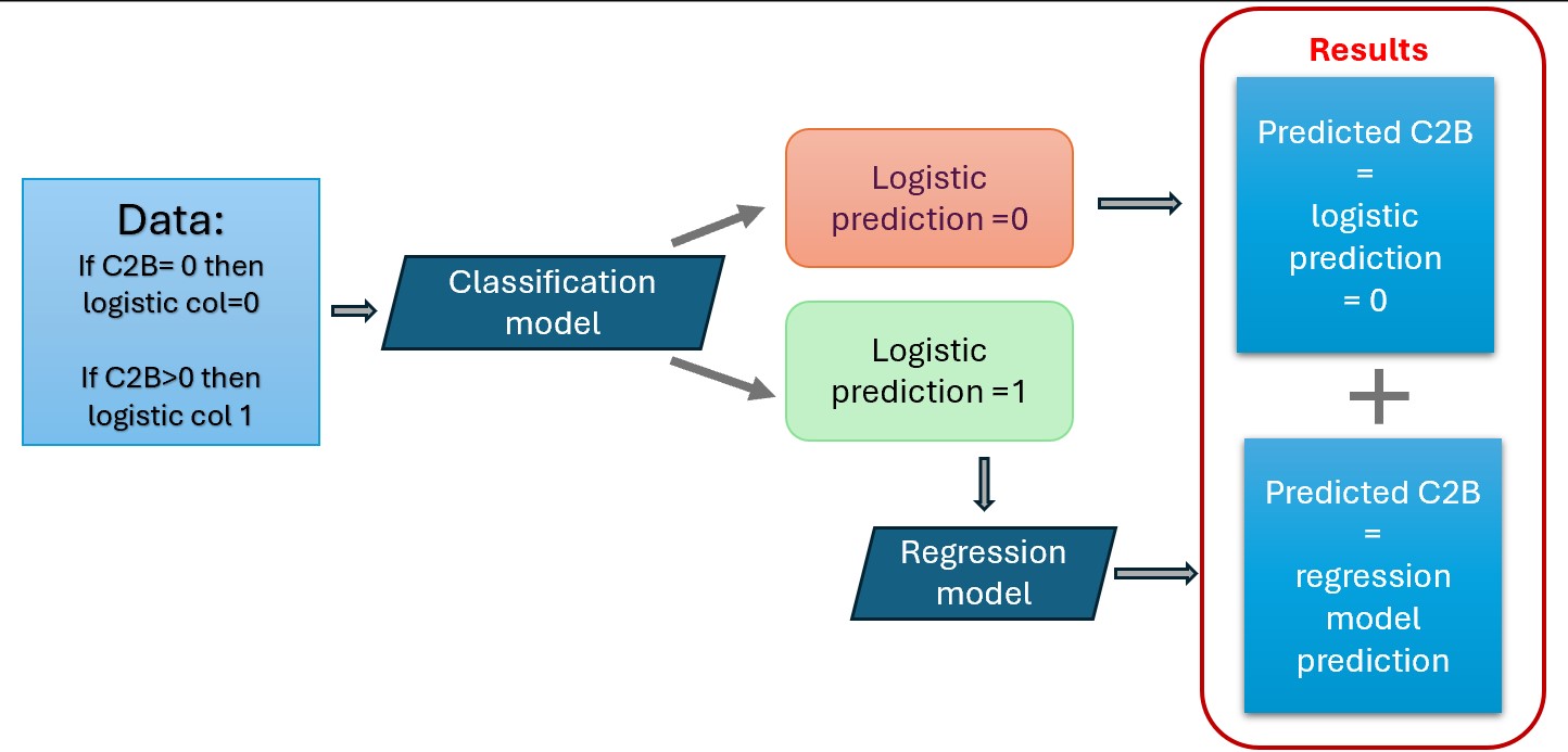
Modelling: Two step approach

For modeling zero-inflated data, I adopted a two-step approach using machine learning techniques tailored to its unique characteristics. Initially, an XGBClassifier identified instances where C2B (conversion rate) exceeded zero, effectively distinguishing between zero and non-zero outcomes. This classifier utilizes gradient boosting for accurate binary predictions.

Subsequently, for non-zero C2B predictions, a regression model was employed to predict the actual conversion rate. This model, often based on linear regression or gradient boosting, aimed to provide precise numerical predictions..

categorical_features = data.select_dtypes(include=['category']).columns.tolist()
print("Categorical Features:", categorical_features)

Categorical Features: ['hotel_id', 'advertiser_id', 'day_of_week', 'stars', 'city_id']

class ML: 
    def __init__(self, data,test_size, num_jobs, random_state):
        print('Machine Learning object is created')
        
        self.data=data
        self.test_size=test_size
        self.num_jobs=num_jobs
        self.random_state = random_state
        # Split the training and test data
        self.X = self.data.drop(['C2B', 'logistic'], axis=1)
        self.y = self.data[['C2B', 'logistic']]
        self.X_train, self.X_test, self.y_train, self.y_test = train_test_split(self.X, self.y, test_size=test_size, random_state=random_state)
        self.y_train_regression = self.y_train[self.y_train['logistic'] == 1]
        self.X_train_regression = self.X_train.loc[self.y_train[self.y_train['logistic'] == 1].index.tolist()]
        # Hyperparameters to tune the models
        self.param_grid = {'n_estimators': [600,800,1000],
                            'learning_rate': [0.01, 0.1],
                            'max_depth': [6,9],
                            'max_leaves': [0,3,6],
                            'colsample_bytree':[0.8]}
   
    def train_classification_model(self):
        # This step is to create the classification model that differentiates the zero from non-zeros in the C2B 
        # using the logistic column as dependent variable
        print('training classification model')
        precision = make_scorer(precision_score, pos_label=1)
        recall = make_scorer(recall_score, pos_label=1)

        scorers = {'precision_score':precision, 'recall_score': recall}#, 'accuracy_score': accuracy_score}
        # Gridsearch with cross validation to fine tuning the model
        classifier = XGBClassifier(random_state=self.random_state, scale_pos_weight=0.8, enable_categorical=True, verbosity=1)
        grid_search_class = GridSearchCV(classifier, self.param_grid, cv=5, n_jobs=self.num_jobs, scoring=scorers, refit='recall_score')
        grid_search_class.fit(self.X_train, self.y_train['logistic'], sample_weight=compute_sample_weight("balanced", self.y_train['logistic']))
        best_params_class = grid_search_class.best_params_
        print('Found best estimastor for classification',  best_params_class)
        # Once that we have the best hyper parameters I train my classification model    
        self.classifier = XGBClassifier(random_state=self.random_state, scale_pos_weight=0.8, enable_categorical=True, verbosity=1,**best_params_class)
        self.classifier.fit(self.X_train, self.y_train['logistic'], sample_weight=compute_sample_weight("balanced", self.y_train['logistic']))
                 
    def train_regression_model(self):
        # This step creates the regression model
        # First: Gridsearch with cross validation to fine tuning the model
        print('training regression model')
        regressor = XGBRegressor(random_state=self.random_state,enable_categorical=True, verbosity=1)
        grid_search = GridSearchCV(regressor, self.param_grid, cv=5, n_jobs=self.num_jobs, scoring='neg_mean_absolute_error')
        grid_search.fit(self.X_train_regression , self.y_train_regression ['C2B'])
        best_params = grid_search.best_params_
        print("Found best estimastor fos regression:", best_params)
        # Once that we have the best hyper parameters I train my regression model  
        self.regressor = XGBRegressor(random_state=self.random_state,enable_categorical=True, verbosity=1, **best_params)
        self.regressor.fit(self.X_train_regression , self.y_train_regression ['C2B'])

    def get_classification_model(self):
        return self.classifier

    def get_regression_model(self):
        return self.regressor

    def evaluate_models(self,plot_scatter=False, plot_residuals=False):
        # This function evaluates the classification and regression models
        if self.classifier and self.regressor:
            #First use x_test to get a y_prediction for the logistic function
            y_pred_class = self.classifier.predict(self.X_test)
            # The predicted class is saved next to y_test data
            self.y_test['predicted_class'] = y_pred_class
            # The rows for which the predicted class is 1 are used in the regression model to get the non-zero C2B
            self.y_test_regressor = self.y_test[self.y_test['predicted_class'] == 1]
            self.X_test_regressor = self.X_test.loc[self.y_test[self.y_test['predicted_class'] == 1].index.tolist()]
            y_pred_reg = self.regressor.predict(self.X_test_regressor)
            self.y_test_regressor['predicted_regression'] = y_pred_reg
            # The predicted regression values are saved in the y test
            self.y_test = pd.merge(self.y_test, self.y_test_regressor[['predicted_regression']], left_index=True, right_index=True, how='outer')
            # If the predicted regression have nan, that means that they correspond to the class 0 predicted with the classification model
            # so I filled the nan with 0s
            self.y_test = self.y_test.fillna(0)
            
            print('Classification evaluation')
            # To evaluate the classification I used the columns logistic and predicted_class in a confusion matrix
            confusion_matrix = pd.crosstab(self.y_test["logistic"], self.y_test["predicted_class"], rownames=["Actual"], colnames=["Predicted"])
            print(confusion_matrix)
            print('recall =', recall_score(self.y_test["logistic"], self.y_test["predicted_class"]))
            
            print('\nRegression evaluation for non zero values')
            # To evaluate the regression, I select all the non zero values from the logistic column, and 
            # the predicted regression values and compute the mean absolute error
            mean_abs_err = np.mean(np.abs(self.y_test[self.y_test['logistic'] == 1]['C2B']- self.y_test[self.y_test['logistic'] == 1]['predicted_regression']))
            print(mean_abs_err)
            if plot_scatter == True:
                # Here I can produce an scatter plot of the true C2B and my predicted value
                plt.figure(figsize=(5,5))
                plt.scatter(self.y_test['C2B'], self.y_test['predicted_regression'])
                plt.xlabel('Actual Values (y-test)')
                plt.ylabel('Predicted Values')
                plt.title('Comparison of Predictions vs. Actual Values')
                plt.xlim(0,100)
                plt.ylim(0,100)
                plt.legend()
                plt.grid(True)
                plt.show()
            if plot_residuals ==True:
                # Here I can visualiza the residuals
                residuals = self.y_test['C2B']-self.y_test['predicted_regression']
                print('Residuals:',residuals.sum())
                plt.figure(figsize=(5,5))
                plt.scatter(self.y_test['predicted_regression'], residuals)
                plt.xlabel('C2B predictions')
                plt.ylabel('Residuals')
                plt.title('Residual Plot')
                plt.axhline(y=0, color='r', linestyle='--')
                plt.show()
            return self.y_test
            
    def visualize_features_importance(self, model='Regression'):
        # This code is to visualize the most important features
        if model!='Regression':
            feature_importance = self.regressor.feature_importances_
        else:
            feature_importance = self.classifier.feature_importances_
        column_names = self.X.columns
        df_feature_importance = pd.DataFrame({'Feature': column_names, 'Importance': feature_importance})
        df_feature_importance = df_feature_importance.sort_values(by='Importance', ascending=False)
        plt.figure(figsize=(7, 4))
        plt.bar(df_feature_importance['Feature'], df_feature_importance['Importance'])
        plt.xlabel('Feature')
        plt.ylabel('Importance')
        plt.title('Feature Importance for '+model)
        plt.xticks(rotation=45, ha='right')
        plt.tight_layout()
        plt.show()

    def fit_new_data(self, X_new):
        # This function is to predict the C2B for new x data
        # Predict classification labels
        y_pred_class = self.classifier.predict(X_new)
        new_data = X_new.copy()
        new_data['predicted_class'] = y_pred_class
        # Select data points predicted as class 1 for regression prediction
        X_new_regression = new_data[new_data['predicted_class'] == 1]
        if not X_new_regression.empty:
            # Predict regression values for class 1 data points
            y_pred_reg = self.regressor.predict(X_new_regression.drop(['predicted_class'], axis=1))
            X_new_regression['predicted_C2B'] = y_pred_reg
            # Merge regression predictions back into the new data
        new_data = pd.merge(new_data, X_new_regression[['predicted_C2B']], left_index=True, right_index=True, how='outer')
        new_data['predicted_C2B'] = new_data['predicted_C2B'].fillna(0)
        return new_data

# Start my object
my_models = ML(data=data,test_size=0.3, random_state=44, num_jobs=2)
# Train classification model
my_models.train_classification_model()
# Train regression model
my_models.train_regression_model()

Machine Learning object is created
training classification model
Found best estimastor for classification {'colsample_bytree': 0.8, 'learning_rate': 0.01, 'max_depth': 6, 'max_leaves': 3, 'n_estimators': 600}
training regression model
Found best estimastor fos regression: {'colsample_bytree': 0.8, 'learning_rate': 0.01, 'max_depth': 6, 'max_leaves': 6, 'n_estimators': 600}

Metrics:

To evaluate model performance, I used:

Recall and Precision: Assessing the classifier's ability to identify non-zero C2B and the accuracy of positive predictions. Mean Absolute Error (MAE): Quantifying the average error magnitude in predicted conversion rates, providing a straightforward measure of regression model accuracy.

These metrics offer insights into model reliability: Recall ensures comprehensive identification of non-zero C2B. Precision minimizes false positives in predicting non-zero C2B.

# Evaluate models
my_models.evaluate_models(plot_scatter=True, plot_residuals=True)

No artists with labels found to put in legend.  Note that artists whose label start with an underscore are ignored when legend() is called with no argument.

Classification evaluation
Predicted     0    1
Actual              
0.0        2063  517
1.0          71  437
recall = 0.860236220472441

Regression evaluation for non zero values
9.75540686771447

Residuals: -7375.6527236122065

	C2B	logistic	predicted_class	predicted_regression
2	0.000000	0.0	0	0.000000
5	0.000000	0.0	0	0.000000
8	6.201550	1.0	1	3.248267
9	2.173913	1.0	1	2.687901
...	...	...	...	...
10274	0.000000	0.0	1	27.453600
10275	0.000000	0.0	1	25.914549
10285	0.000000	0.0	1	31.652863
10290	5.882353	1.0	1	28.232504

3088 rows × 4 columns

# Visualiza features
my_models.visualize_features_importance(model='Classification')
my_models.visualize_features_importance(model='Regression')

#Make predictions for day 11
day_11_with_prediction = my_models.fit_new_data(data_day_11.drop(['C2B', 'logistic'], axis=1))
day_11_with_prediction

	hotel_id	advertiser_id	day_of_week	n_clickouts_lag_1d	n_clickouts_lag_3d_a	n_clickouts_lag_3d_sd	n_clickouts_lag_perc_change	n_bookings_lag_1d	n_bookings_lag_3d_a	n_bookings_lag_3d_sd	...	C2B_lag_3d_a	C2B_lag_3d_sd	C2B_lag_perc_change	probability_of_booking	stars	n_reviews	rating	city_id	predicted_class	predicted_C2B
0	1	1	Friday	1.0	2.000000	1.732051	-0.750000	0.0	0.000000	0.000000	...	0.000000	0.000000	NaN	0.000000	3	3601.0	6.1	36	0	0.000000
1	1	5	Friday	103.0	135.000000	30.199338	-0.258993	4.0	4.666667	4.041452	...	3.374797	2.441106	4.398058	1.000000	3	3601.0	6.1	36	1	2.687901
2	1	14	Friday	1.0	1.000000	0.000000	0.000000	0.0	0.000000	0.000000	...	0.000000	0.000000	NaN	0.000000	3	3601.0	6.1	36	0	0.000000
3	1	37	Friday	1.0	4.333333	3.511885	-0.875000	0.0	0.000000	0.000000	...	0.000000	0.000000	NaN	0.000000	3	3601.0	6.1	36	0	0.000000
...	...	...	...	...	...	...	...	...	...	...	...	...	...	...	...	...	...	...	...	...	...
2036	186	37	Friday	45.0	22.666667	19.399313	2.461538	0.0	0.000000	0.000000	...	0.000000	0.000000	NaN	0.250000	3	709.0	7.5	44	1	22.782862
2037	186	17	Friday	14.0	7.666667	6.027714	1.000000	0.0	0.000000	0.000000	...	0.000000	0.000000	NaN	0.142857	3	709.0	7.5	44	0	0.000000
2038	186	24	Friday	17.0	8.666667	7.371115	1.833333	1.0	0.666667	0.577350	...	13.071895	17.791709	NaN	0.285714	3	709.0	7.5	44	1	23.193806
2039	186	14	Friday	2.0	NaN	NaN	NaN	1.0	NaN	NaN	...	NaN	NaN	NaN	1.000000	3	709.0	7.5	44	1	43.095139

2040 rows × 22 columns